深度学习-10

参数管理

访问参数，用于调试、诊断和可视化。
参数初始化。
在不同模型组件间共享参数

参数访问

用Sequential类定义模型，可通过索引来访问模型的任一层
模型像一个列表，每层的参数在其属性中

目标参数

每个参数都表示为参数类的一个实例
要对参数执行任何操作，首先要访问底层的数值
可以访问权重、偏置、梯度等参数

一次性访问所有参数：

第一种：

1 2	print([(name, param.shape) for name, param in net[0].named_parameters()]) print([(name, param.shape) for name, param in net.named_parameters()])

第二种：

1	net.state_dict()['2.bias'].data

从嵌套块收集参数

def block1():
    return nn.Sequential(nn.Linear(4, 8), nn.ReLU(),
                         nn.Linear(8, 4), nn.ReLU())

def block2():
    net = nn.Sequential()
    for i in range(4):
        # 在这里嵌套
        net.add_module(f'block {i}', block1())
    return net

rgnet = nn.Sequential(block2(), nn.Linear(4, 1))
rgnet(X)

Sequential(
  (0): Sequential(
    (block 0): Sequential(
      (0): Linear(in_features=4, out_features=8, bias=True)
      (1): ReLU()
      (2): Linear(in_features=8, out_features=4, bias=True)
      (3): ReLU()
    )
    (block 1): Sequential(
      (0): Linear(in_features=4, out_features=8, bias=True)
      (1): ReLU()
      (2): Linear(in_features=8, out_features=4, bias=True)
      (3): ReLU()
    )
    (block 2): Sequential(
      (0): Linear(in_features=4, out_features=8, bias=True)
      (1): ReLU()
      (2): Linear(in_features=8, out_features=4, bias=True)
      (3): ReLU()
    )
    (block 3): Sequential(
      (0): Linear(in_features=4, out_features=8, bias=True)
      (1): ReLU()
      (2): Linear(in_features=8, out_features=4, bias=True)
      (3): ReLU()
    )
  )
  (1): Linear(in_features=4, out_features=1, bias=True)
)

参数初始化

内置初始化

下面的代码将所有权重参数初始化为标准差为0.01的高斯随机变量，且将偏置参数设置为0。

def init_normal(m):
    if type(m) == nn.Linear:
        nn.init.normal_(m.weight, mean=0, std=0.01)
        // 也可以给定常数
        //nn.init.constant_(m.weight, 1)
        nn.init.zeros_(m.bias)
net.apply(init_normal)
net[0].weight.data[0], net[0].bias.data[0]

自定义初始化

def my_init(m):
    if type(m) == nn.Linear:
        print("Init", *[(name, param.shape)
                        for name, param in m.named_parameters()][0])
        nn.init.uniform_(m.weight, -10, 10)
        m.weight.data *= m.weight.data.abs() >= 5

net.apply(my_init)
net[0].weight[:2]

net[0].weight.data[:] += 1
net[0].weight.data[0, 0] = 42
net[0].weight.data[0]

参数绑定

在多个层间共享参数

定义一个稠密层，然后使用它的参数来设置另一个层的参数。

# 我们需要给共享层一个名称，以便可以引用它的参数。
shared = nn.Linear(8, 8)
net = nn.Sequential(nn.Linear(4, 8), nn.ReLU(),
                    shared, nn.ReLU(),
                    shared, nn.ReLU(),
                    nn.Linear(8, 1))
net(X)
# 检查参数是否相同
print(net[2].weight.data[0] == net[4].weight.data[0])
net[2].weight.data[0, 0] = 100
# 确保它们实际上是同一个对象，而不只是有相同的值。
print(net[2].weight.data[0] == net[4].weight.data[0])

共享参数的好处：

共享参数通常可以节省内存，并在以下方面具有特定的好处：

对于图像识别中的CNN，共享参数使网络能够在图像中的任何地方而不是仅在某个区域中查找给定的功能。
对于RNN，它在序列的各个时间步之间共享参数，因此可以很好地推广到不同序列长度的示例。
对于自动编码器，编码器和解码器共享参数。在具有线性激活的单层自动编码器中，共享权重会在权重矩阵的不同隐藏层之间强制正交。

延后初始化--defers initialization

框架的延后初始化（defers initialization），即等到我们第一次将数据通过模型传递时，才会动态地推断出每个层的大小。

import tensorflow as tf

net = tf.keras.models.Sequential([
    tf.keras.layers.Dense(256, activation=tf.nn.relu),
    tf.keras.layers.Dense(10),
])

自定义层

不带参数的层

import torch
import torch.nn.functional as F
from torch import nn


class CenteredLayer(nn.Module):
    def __init__(self):
        super().__init__()

    def forward(self, X):
        return X - X.mean()

带参数的层

class MyLinear(nn.Module):
    def __init__(self, in_units, units):
        super().__init__()
        self.weight = nn.Parameter(torch.randn(in_units, units))
        self.bias = nn.Parameter(torch.randn(units,))
    def forward(self, X):
        linear = torch.matmul(X, self.weight.data) + self.bias.data
        return F.relu(linear)

读写文件

加载和保存张量

import torch
from torch import nn
from torch.nn import functional as F

x = torch.arange(4)
torch.save(x, 'x-file')

加载和保存模型参数

class MLP(nn.Module):
    def __init__(self):
        super().__init__()
        self.hidden = nn.Linear(20, 256)
        self.output = nn.Linear(256, 10)

    def forward(self, x):
        return self.output(F.relu(self.hidden(x)))

net = MLP()
X = torch.randn(size=(2, 20))
Y = net(X)

# 存储文件
torch.save(net.state_dict(), 'mlp.params')

# 直接读取文件中存储的参数
clone = MLP()
clone.load_state_dict(torch.load('mlp.params'))
clone.eval()

MLP(
  (hidden): Linear(in_features=20, out_features=256, bias=True)
  (output): Linear(in_features=256, out_features=10, bias=True)
)

GPU

计算设备

在PyTorch中，CPU和GPU可以用torch.device('cpu')和torch.cuda.device('cuda')表示。
cpu设备意味着所有物理CPU和内存。这意味着PyTorch的计算将尝试使用所有CPU核心。
gpu设备只代表一个卡和相应的显存。如果有多个GPU
使用torch.cuda.device(f'cuda:{i}')来表示第i块GPU（i从0开始）
cuda:0和cuda是等价的。

import torch
from torch import nn

torch.device('cpu'), torch.cuda.device('cuda'), torch.cuda.device('cuda:1')

查询GPU的数量

1	torch.cuda.device_count()

请求GPU

def try_gpu(i=0):  #@save
    """如果存在，则返回gpu(i)，否则返回cpu()。"""
    if torch.cuda.device_count() >= i + 1:
        return torch.device(f'cuda:{i}')
    return torch.device('cpu')

def try_all_gpus():  #@save
    """返回所有可用的GPU，如果没有GPU，则返回[cpu(),]。"""
    devices = [torch.device(f'cuda:{i}')
             for i in range(torch.cuda.device_count())]
    return devices if devices else [torch.device('cpu')]

try_gpu(), try_gpu(10), try_all_gpus()

这两个函数允许我们在请求的GPU不存在的情况下运行代码

张量与gpu

默认情况下，张量是在CPU上创建的。

查询张量所在的设备:

x.ctx

存储在GPU上

1 2	X = np.ones((2, 3), ctx=try_gpu()) X

第二个GPU上创建一个随机张量

1 2	Y = np.random.uniform(size=(2, 3), ctx=try_gpu(1)) Y

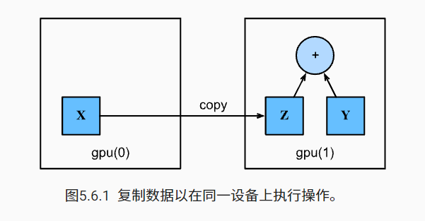
复制

计算X+Y，可以将X传输到第二个GPU进行操作

1
2
3

Z = X.copyto(try_gpu(1))
print(X)
print(Z)

只想在变量存在于不同设备中时进行复制。在这种情况下，我们可以调用as_in_ctx。
如果变量已经存在于指定的设备中，则这不会进行任何操作。除非你特别想创建一个复制，否则选择as_in_ctx方法。

1	Z.as_in_ctx(try_gpu(1)) is Z

神经网络与GPU

神经网络模型可以指定设备

1 2	net = nn.Sequential(nn.Linear(3, 1)) net = net.to(device=try_gpu())

小结

我们可以指定用于存储和计算的设备，例如CPU或GPU。默认情况下，数据在主内存中创建，然后使用CPU进行计算。
深度学习框架要求计算的所有输入数据都在同一设备上，无论是CPU还是GPU。
不经意地移动数据可能会显著降低性能。一个典型的错误如下：计算GPU上每个小批量的损失，并在命令行中将其报告给用户（或将其记录在NumPy ndarray中）时，将触发全局解释器锁，从而使所有GPU阻塞。最好是为GPU内部的日志分配内存，并且只移动较大的日志。